Wolfram Mathematica 14.3.0

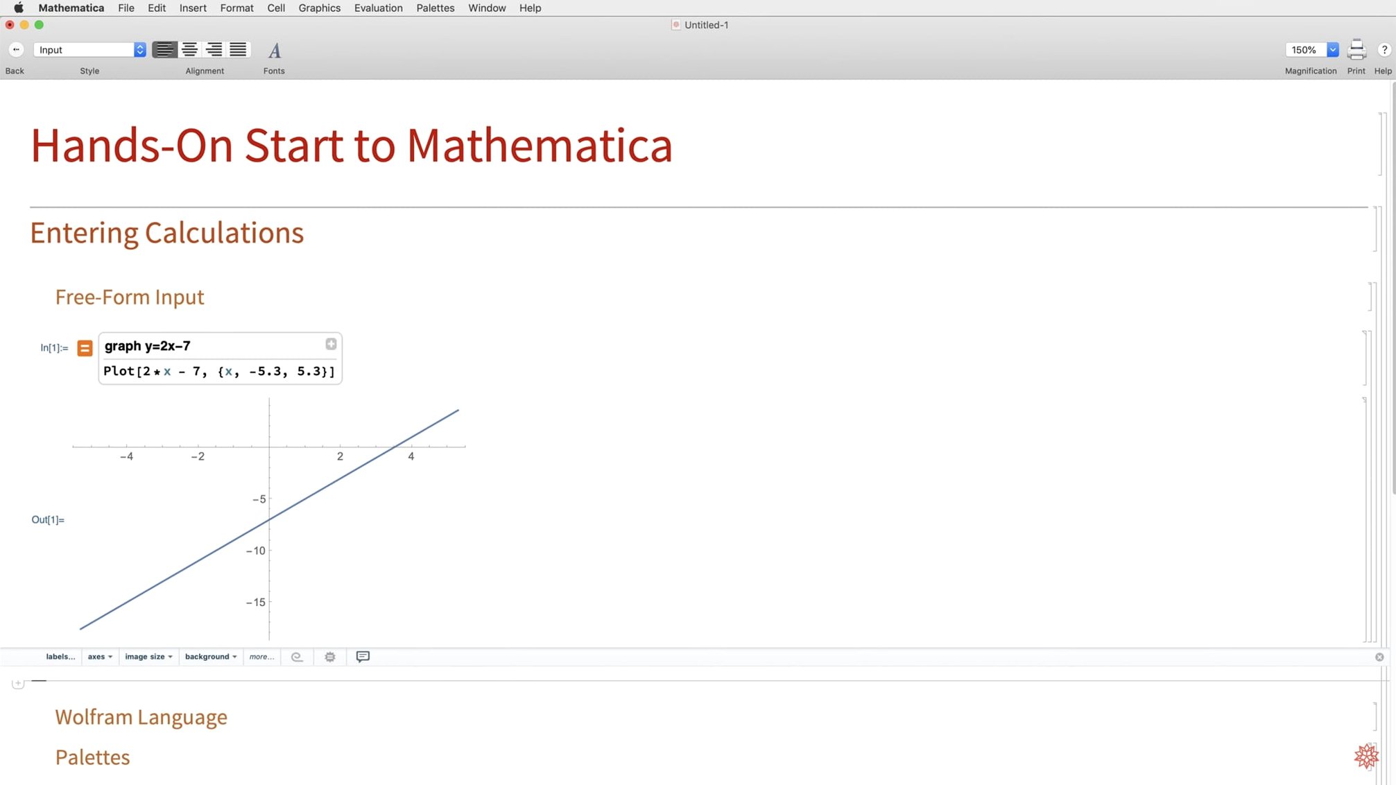
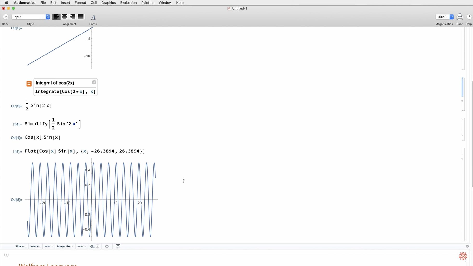
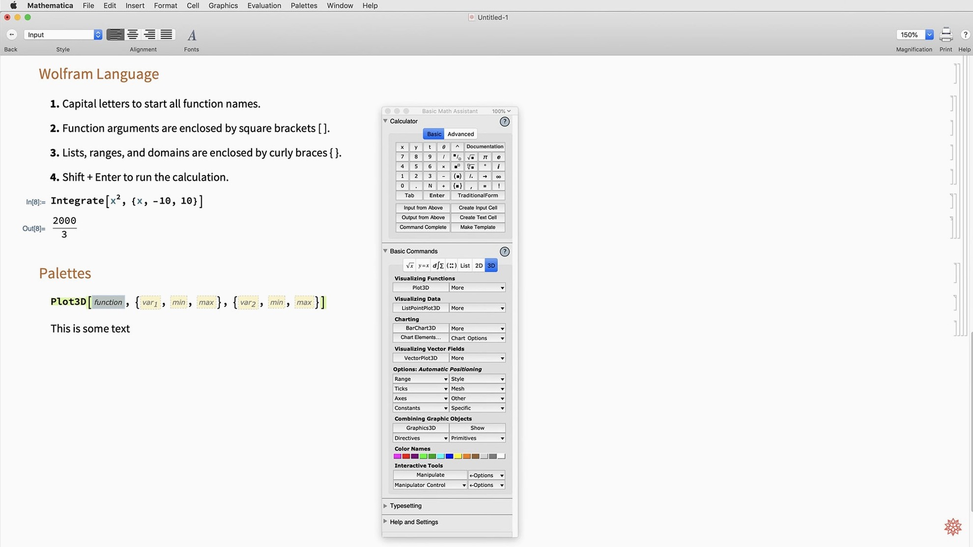
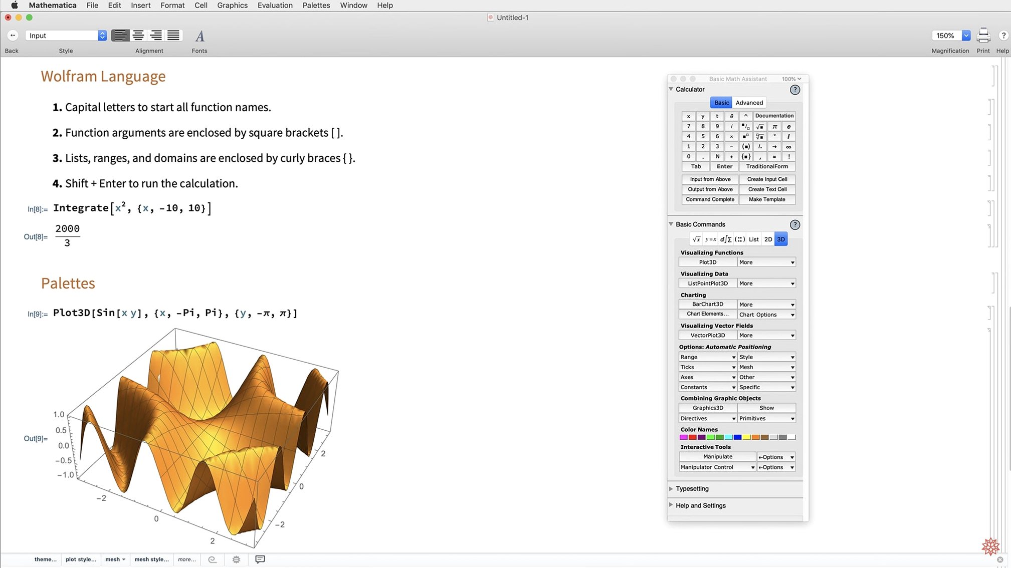
Thousands of built-in Wolfram Language functions ship with Mathematica, covering everything from basic algebra to neural network construction. It arrives on your Mac not as a single-purpose calculator, but as a complement to the spreadsheet, the text editor, and the presentation tool you already use daily.

Symbolic derivation alongside your word processor

Type an equation with natural-language input, get a fully formatted symbolic result, then paste a high-resolution rendering straight into a Pages or Word document. No LaTeX boilerplate needed.

Numerical analysis that feeds your spreadsheets

Pull external data from a CSV or database, run a Hilbert transform on it, and deploy the result in the format you need. Mathematica handles the heavy maths that a spreadsheet formula column simply cannot.

Visualisation ready for Keynote or PowerPoint

Build a vector-based map or a ListFitPlot, style it with the new standard dark-mode colours, then export it as a crisp graphic for your next presentation. It lands on the slide as native artwork, not a screenshot.

Small conveniences that repay a moment's curiosity

Mathematica rewards the habit of pausing to right-click. A Control-click on almost any output reveals a context menu with a "Make Template" option — an instant way to turn a successful calculation into a reusable function without retyping a single bracket. Similarly, if you find yourself adjusting a slider in a Manipulate pane and wish you could nudge it with the keyboard, know that arrow keys step through discrete values while holding Shift speeds up the increment. These tiny shortcuts are rarely the first thing a new user discovers, but they quietly reshape a working session once you know they exist.

A few others worth filing away: Cmd-Shift-Enter evaluates an entire notebook in one pass, ideal when you reopen yesterday’s work and want every cell to recalculate in sequence. The new dark mode, introduced in version 14.3, is not just a palette swap; it respects the notebook’s syntax colouring and can be toggled per document from the bottom toolbar, so you can keep a bright white computational essay open while the main coding notebook stays in a low-glare dark scheme. And for anyone who regularly types Wolfram Language, the automatic template completion — triggered by typing a function name and pressing Cmd-Shift-K — can fill in the argument structure before you forget what order the parameters expect.

Typing loose integral descriptions and letting the parser propose symbolic form

Imagine a Tuesday afternoon. You open Mathematica with a fresh notebook and start by typing a loose description: “integrate sin of x squared times cosine of x.” The natural-language interpreter offers a precise symbolic input, which you accept with a tap of the Return key. The result appears in a fraction of a second, rendered in clear mathematical notation. You spot a pattern worth investigating, so you highlight the output, right-click, and choose Make Template. A new function definition appears, and you tweak the argument names to suit the problem you are actually solving.

Next, you pull in a CSV of experimental data dropped onto the Dock icon. A ListPlot call gives you a rough scatter plot. You then wrap it in ListFitPlot, introduced in 14.3, and immediately see a fitted curve overlaid on the raw points. The plot looks useful, but the default colours feel a little loud for the report you are drafting. You open the new colour chooser, switch to the standard dark-mode palette, and pick a muted teal and slate combination that will print cleanly in greyscale. A quick Cmd-C copies the graphic as a vector, and you paste it into your Pages document without breaking stride.

Before closing the notebook, you run Cmd-Shift-Enter to re-evaluate everything from top to bottom. The cells hum through their calculations, and you save the notebook knowing it will open tomorrow in exactly the state you left it. Total elapsed time: perhaps twenty-five minutes, most of it spent thinking rather than wrestling with tooling.

A data analyst's real-world morning

Consider someone who spends their days wrangling survey results in a research unit. The raw data arrives as a CSV with a dozen columns of Likert-scale responses and demographic tags. Opening it in a spreadsheet is the obvious move until the question arises: “Are the response distributions for the under-25 group significantly different from the over-60 group?” A spreadsheet can give you averages, but it will not compute a Kolmogorov–Smirnov test without add-ons, nor will it show you the kernel density estimates side by side.

This analyst drags the CSV into Mathematica, assigns it to a variable with a single SemanticImport call, and filters the age groups with a one-line Wolfram Language query. Two density plots appear stacked vertically in the output, styled in the new dark-mode colours so they read clearly on a projector during the afternoon meeting. The K-S test result sits beneath them, formatted as a tidy table. The whole workflow — import, filter, test, plot — fits inside a dozen lines of code and a single notebook. When a colleague asks for the underlying numbers, the analyst exports the table as Markdown, a format newly supported in 14.3, and pastes it into the team’s shared notes without reformatting. Nothing was photographed off the screen, nothing was re-typed, and the notebook remains a self-contained record of every statistical decision made that morning.

Daily use differences with MATLAB, Maple, and command-line Python

Mathematica shares shelf space with a handful of heavyweight computational environments, and the differences are worth understanding in terms of daily use rather than feature checklists.

MATLAB is the comparison most engineers make first. MATLAB excels at matrix operations and has a vast Simulink ecosystem for control systems and signal processing. Its language is procedural and linear-algebra-first; you work with matrices as the fundamental data type. Mathematica, by contrast, treats everything as a symbolic expression — a matrix is just one kind of expression among many. That means you can differentiate a function symbolically and then numerically integrate the result in the same notebook without switching toolboxes. The trade-off is that MATLAB’s large-scale numerical linear algebra can feel more direct for certain engineering workflows, while Mathematica’s symbolic core makes it the natural choice when the problem starts with an equation rather than a dataset.

Maple is the closest cousin in spirit, another symbolic engine with strong visualisation. Maple’s interface has historically felt more document-like, with a clickable math palette that appeals to undergraduates. Mathematica’s notebook interface is more programmable in its own right — you can build interactive dashboards with Manipulate that would require a separate GUI toolkit in Maple. Both handle symbolic integration and differential equations fluently, but Mathematica’s breadth across data science, image processing, and even natural-language querying gives it a broader remit once you move beyond pure calculus.

Python with Jupyter (often via Anaconda) is the open-source contender. A Jupyter notebook running NumPy, SymPy, and Matplotlib can mimic many of Mathematica’s capabilities, and it costs nothing to install. The friction arises in integration: SymPy for symbolic work, NumPy for numerics, Matplotlib for plots, and Pandas for data frames are separate libraries with different syntax conventions. Mathematica wraps all those domains in one consistent language and one notebook format. The trade-off is that Python’s ecosystem connects more readily to web frameworks and production servers, while Mathematica tends to be the place where prototyping and deep exploration happen before anything gets deployed elsewhere.

Wolfram Mathematica 14.3 embraces the look of modern macOS with full dark mode support and a carefully tuned set of standard colours for both light and dark environments. The update also broadens the mathematical toolkit with Hilbert transforms, Lommel functions, and new matrix decompositions. On the visualisation side, ListFitPlot, surface plotting additions, vector-based maps, and mesh processing tools give you more ways to explore data. Under the hood, geodesic computation, LLMGraph, speedier Python and R integration, ColumnwiseCombine, system model validation tools, and Markdown export support round out the release.

• macOS 12 or later
• Apple Silicon or Intel Mac